Matrix Population Models (MPMs)
by Iain Stott

Matrix Population Models (MPMs) are one of the most widely-used modelling tools in population ecology. Many projects and studies have used MPM models to inform on population management strategies for conservation (Esparza-Olguin et al. 2002 Biol. Conserv. 103 349-359; Linares et al. 2007 Ecology 88 918-928), pest control and invasive species (Dudas, Dower and Anholt 2007 Ecology 88 2084-2093) and harvesting (Cropper and DiResta 1999 Ecol. Model. 118 1-15), amongst other applications. The main thing that differentiates matrix models from earlier population models is the ability to incorporate vital rates that are heterogeneous across the life cycle. Earlier models (Lotka-Volterra models being the classic example) assumed that each individual in the population was equal to every other in their contribution, whereas we know this is not the case. For example, juveniles have differing reproductive contributions to adults, survival may depend on age or size, growth rate may depend on geographic location or genotype, and so on.

Life Cycles and Matrix Population Models
by Iain Stott

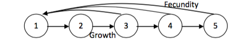
At the core of the MPM model is the life cycle. This describes how each stage of life is connected to each other stage. The simplest example of a life cycle is one structured by age. Each individual grows to the next age class every year, and adults give birth to young:

However, many organisms do not conform to a rigid age-structured life. For many, there are distinct stages of life that may be independent of age (such as for insects with a larva-pupa-adult life cycle) and for others, their survival and reproduction may depend on other aspects of their biology (for example, plant fecundity is often dictated by size rather than age). In such cases, a stage-structured life cycle may be more appropriate. In a stage-structured life cycle, movement between life stages is more complex, in addition to growing and reproducing, individuals may stay in their current stage class (stasis), skip stage classes (progression) or regress back through the life cycle (regression):

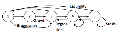
Numbers can be attached to the arrows in such life cycles: these represent the contributions that each stage class makes to each other stage class. For example, stage 4 in the above cycle might have a stasis of 0.2, a growth of 0.4, a regression of 0.1 and a fecundity of 2. This means that on average, in a given year, 20% of individuals stay as a stage 4 (e.g. if the organism was a plant and the life cycle is size-based, they do not get any smaller or larger) 40% become a stage 5 (e.g. they grow larger), 10% become a stage 3 (e.g. they get smaller, perhaps because of herbivory) and 2 seedlings germinate and survive and are recruited to the population.
This is where the MPM comes in: to represent these life cycle graphs in a mathematical format, we present the life cycle as a matrix. Each column represents the current stage class an individual may be in, and each row represents the stage class that those individuals may move into. The vital rates are placed in their corresponding positions in the matrix:

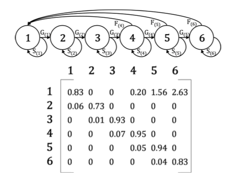
The columns represent the current stage and the rows represent the stage in the next time interval. So, G(1)=growth of stage 1 into stage 2 with probability 0.06. S(4)=Stasis of stage 4 with probability 0.95. F(6)=fecundity of stage 6, contributing on average 2.63 offspring to the subsequent year. This matrix is in fact for a palm, Iriartea deltoidea (Pinard 1993 Biotropica 25 2-14). The earliest PPM models were age-structured, called Leslie matrices after P. H. Leslie, who introduced them to ecology. Stage-structured models are often called Lefkovitch matrices, after L. P. Lefkovitch. These broad classifications are often made more specific nowadays, according to whether, in addition to the ubiquitous growth and fecundity rates, they include stasis, progression and/or regression through the life cycle (Carslake 2009 Ecology 90 3258-3267).

Additional Information

For the purposes of matrix modelling, life cycles are often considered to have a number of specific mathematical properties. These are related to the Perron-Frobenius strong ergodic theorem, pertaining to the asymptotic (i.e. long-term) predictions of the model. Specifically, matrices are often assumed to be irreducible and primitive. As well as having considerable mathematical consequences for analysis, irreducibility and primitivity are often key to a biologically rational life cycle, but may arise as a consequence of methodologies in data collection – see (Stott et al. 2010 Methods Ecol. Evol. 1 242-252) for more details.